Tutorial - Part 1

This tutorial will walk you through the steps of designing and running a simple Phantom experiment. It is based on the included supply_chain.py example that can be found in the examples/environments/supply_chain directory in the Phantom repo.

Experiment Goals

We want to model a very simple supply chain consisting of three types of agents: factories, shops and customers. Our supply chain has one product that is available in whole units. We do not concern ourselves with prices or profits here.

Factory Agent

The factory is a simple agent in this environment. The shop can make unlimited requests for stock to the factory. The factory holds unlimited stock and will always completely fulfil the shop’s requests.

It does not have a policy, or make actions and observations. It simply reacts to the actions of other agents via the messages (requests for stock) it receives. Because of this we use the Agent class and not the StrategicAgent class.

Customer Agent

The customer agents do take an active role by creating order requests to the shop. Every step they make an order for a variable quantity of product. In this tutorial we sample a value from a random distribution to get the quantity requested. Because of this the customer does not need to make observations and hence we can still make use of the Agent class and its generate_messages() method.

We model the number of products requested with a Poisson random distribution. As there is only one shop the customers will always visit the same shop. Customers receive products from the shop after making an order. We do not need to do anything with this when received.

Shop Agent

The shop is the only learning agent in this experiment. It makes observations, queries its policy and takes actions from this. As such we use the StrategicAgent class to create the shop.

The shop can only hold a fixed amount of inventory and as such can only make a request of this size to the factory for more stock. It receives orders from customers and will fulfil these orders as best it can.

The shop takes one action each step - the request for more stock that it sends to the factory. The amount it requests is decided by the policy. The policy is informed by several observations: TODO.

The goal is for the shop to learn a policy where it requests a suitable amount of stock requests to the factory each step so that it can fulfil all it’s orders without holding onto too much unecessary stock. This goal is implemented in the shop agent’s reward function, we reward for sales made and penalise for excess stock held.

Implementation

First we import the libraries we require and define some constants.

from dataclasses import dataclass

import gymnasium as gym
import numpy as np
import phantom as ph


NUM_EPISODE_STEPS = 100

NUM_CUSTOMERS = 5
CUSTOMER_MAX_ORDER_SIZE = 5
SHOP_MAX_STOCK = 100

As this experiment is simple we can easily define it entirely within one file. For more complex, larger experiments it is recommended to split the code into multiple files, making use of the modularity of Phantom.

Next we define message payload classes for each type of message. This helps to enforce the type of information that is sent between agents and can help reduce bugs in complex environments. The message payload classes are frozen, or immutable, which means once created they cannot be modified in transport.

@dataclass(frozen=True)
class OrderRequest(ph.MsgPayload):
    """Customer --> Shop"""
    size: int


@dataclass(frozen=True)
class OrderResponse(ph.MsgPayload):
    """Shop --> Customer"""
    size: int


@dataclass(frozen=True)
class StockRequest(ph.MsgPayload):
    """Shop --> Factory"""
    size: int


@dataclass(frozen=True)
class StockResponse(ph.MsgPayload):
    """Factory --> Shop"""
    size: int

Next, for each of our agent types we define a new Python class that encapsulates all the functionality the given agent needs:

Factory Agent

The factory is the simplest to implement as it does not take actions and does not store state. We inherit from the Agent class:

class FactoryAgent(ph.Agent):
    def __init__(self, agent_id: str):
        super().__init__(agent_id)

We define the functionality for handling messages with ph.agents.msg_handler decorated methods. Each method handles a different type of message as given to the decorator:

    @ph.agents.msg_handler(StockRequest)
    def handle_stock_request(self, ctx: ph.Context, message: ph.Message):
        # The factory receives stock request messages from shop agents. We simply
        # reflect the amount of stock requested back to the shop as the factory can
        # produce unlimited stock.
        return [(message.sender_id, StockResponse(message.payload.size))]

#

Here we take any stock request we receive from the shop (the payload of the message) and reflect it back to the shop as the factory will always completely fulfil any stock request it receives.

Customer Agent

The implementation of the customer agent class takes more work as it stores state and generates its own messages.

We take the ID of the shop as an initialisation parameter and store it as local state. It is recommended to always handle IDs this way rather than hard-coding them.

class CustomerAgent(ph.Agent):
    def __init__(self, agent_id: ph.AgentID, shop_id: ph.AgentID):
        super().__init__(agent_id)

        # We need to store the shop's ID so we know who to send order requests to.
        self.shop_id: str = shop_id

    @ph.agents.msg_handler(OrderResponse)
    def handle_order_response(self, ctx: ph.Context, message: ph.Message):
        # The customer will receive it's order from the shop but we do not need to
        # take any actions on it.
        return

    def generate_messages(self, ctx: ph.Context):
        # At the start of each step we generate an order with a random size to send
        # to the shop.
        order_size = np.random.randint(CUSTOMER_MAX_ORDER_SIZE)

        # We perform this action by sending a stock request message to the factory.
        return [(self.shop_id, OrderRequest(order_size))]

The generate_messages(), decode_action() and any message handler method can all return new messages to deliver. These can be to any other agent that the agent is connected to. This is done by optionally returning a list of tuples with each tuple containing the ID of the agent to send to and the message contents.

Shop Agent

As the learning agent in our experiment, the shop agent is the most complex and introduces some new features of Phantom. As seen below, we store more local state than before. Note that we inherit from StrategicAgent and not Agent as before.

We keep track of sales and missed sales for each step.

class ShopAgent(ph.StrategicAgent):
    def __init__(self, agent_id: str, factory_id: str):
        super().__init__(agent_id)

        # We store the ID of the factory so we can send stock requests to it.
        self.factory_id: str = factory_id

        # We keep track of how much stock the shop has...
        self.stock: int = 0

        # ...and how many sales have been made...
        self.sales: int = 0

        # ...and how many sales per step the shop has missed due to not having enough
        # stock.
        self.missed_sales: int = 0

        # = [Stock, Sales, Missed Sales]
        self.observation_space = gym.spaces.Box(low=0.0, high=1.0, shape=(3,))

        # = [Restock Quantity]
        self.action_space = gym.spaces.Box(low=0.0, high=SHOP_MAX_STOCK, shape=(1,))

We want to keep track of how many sales and missed sales we made in the step. When messages are sent, the shop will start taking orders. So before this happens we want to reset our counters. We can do this by defining a pre_message_resolution() method. This is called directly before messages are sent across the network in each step.

    def pre_message_resolution(self, ctx: ph.Context):
        # At the start of each step we reset the number of missed orders to 0.
        self.sales = 0
        self.missed_sales = 0
#

We define two message handler methods: one for handling order requests from customers and one for handling stock deliveries from the factory.

    @ph.agents.msg_handler(StockResponse)
    def handle_stock_response(self, ctx: ph.Context, message: ph.Message):
        # Messages received from the factory contain stock.
        self.delivered_stock = message.payload.size

        self.stock = min(self.stock + self.delivered_stock, SHOP_MAX_STOCK)

    @ph.agents.msg_handler(OrderRequest)
    def handle_order_request(self, ctx: ph.Context, message: ph.Message):
        amount_requested = message.payload.size

        # If the order size is more than the amount of stock, partially fill the order.
        if amount_requested > self.stock:
            self.missed_sales += amount_requested - self.stock
            stock_to_sell = self.stock
            self.stock = 0
        # ... Otherwise completely fill the order.
        else:
            stock_to_sell = amount_requested
            self.stock -= amount_requested

        self.sales += stock_to_sell

        # Send the customer their order.
        return [(message.sender_id, OrderResponse(stock_to_sell))]

#

We encode the shop’s observation with the encode_observation() method. In this we apply some simple scaling to the values.

    def encode_observation(self, ctx: ph.Context):
        max_sales_per_step = NUM_CUSTOMERS * CUSTOMER_MAX_ORDER_SIZE

        return np.array(
            [
                self.stock / SHOP_MAX_STOCK,
                self.sales / max_sales_per_step,
                self.missed_sales / max_sales_per_step,
            ],
            dtype=np.float32,
        )
#

We define a decode_action() method for taking the action from the policy and translating it into messages to send in the environment. Here the action taken is making requests to the factory for more stock. As we have set the action space to be continuous we need to convert the action to an integer value as we only deal with whole units of stock.

    def decode_action(self, ctx: ph.Context, action: np.ndarray):
        # The action the shop takes is the amount of new stock to request from
    # the factory, clipped so the shop never requests more stock than it can hold.
    stock_to_request = min(int(round(action[0])), SHOP_MAX_STOCK - self.stock)

        # We perform this action by sending a stock request message to the factory.
        return [(self.factory_id, StockRequest(stock_to_request))]
#

Next we define a compute_reward() method. Every step we calculate a reward based on the agents current state in the environment and send it to the policy so it can learn a good policy.

    def compute_reward(self, ctx: ph.Context) -> float:
        # We reward the agent for making sales.
        # We penalise the agent for holding onto excess stock.
        return self.sales - 0.1 * self.stock
#

Each episode can be thought of as a completely independent trial for the environment. However creating a new environment each time with a new network, agents could potentially slow our simulations down a lot. Instead we can reset our objects back to an initial state. This is done with the reset() method:

    def reset(self):
        self.stock = 0
#

Environment

Now we have defined all our agents and their behaviours we can describe how they will all interact by defining our environment. Phantom provides a base PhantomEnv class that the user should create their own class and inherit from. The PhantomEnv class provides a default set of required methods such as step() which coordinates the evolution of the environment for each episodes.

Advanced users of Phantom may want to implement advanced functionality and write their own methods, but for most simple use cases the provided methods are fine. The minimum a user needs to do is define a custom initialisation method that defines the network and the number of episode steps.

class SupplyChainEnv(ph.PhantomEnv):
    def __init__(self):

The recommended design pattern when creating your environment is to define all the agent IDs up-front and not use hard-coded values:

        # Define agent IDs
        factory_id = "WAREHOUSE"
        customer_ids = [f"CUST{i+1}" for i in range(NUM_CUSTOMERS)]
        shop_id = "SHOP"
#

Next we define our agents by creating instances of the classes we previously wrote:

        factory_agent = FactoryAgent(factory_id)
        customer_agents = [CustomerAgent(cid, shop_id=shop_id) for cid in customer_ids]
        shop_agent = ShopAgent(shop_id, factory_id=factory_id)

#

Then we accumulate all our agents into one list so we can add them to the network. We then use the IDs to create the connections between our agents:

        agents = [shop_agent, factory_agent] + customer_agents

        # Define Network and create connections between Actors
        network = ph.Network(agents)

        # Connect the shop to the factory
        network.add_connection(shop_id, factory_id)

        # Connect the shop to the customers
        network.add_connections_between([shop_id], customer_ids)
#

Finally we make sure to initialise the parent PhantomEnv class:

        super().__init__(num_steps=NUM_EPISODE_STEPS, network=network)
#

Metrics

Before we start training we add some basic metrics to help monitor the training progress. These will be described in more detail in the second part of the tutorial.

metrics = {
    "SHOP/stock": ph.metrics.SimpleAgentMetric("SHOP", "stock", "mean"),
    "SHOP/sales": ph.metrics.SimpleAgentMetric("SHOP", "sales", "mean"),
    "SHOP/missed_sales": ph.metrics.SimpleAgentMetric("SHOP", "missed_sales", "mean"),
}

Training the Agents

Training the agents is done by making use of one of RLlib’s many reinforcement learning algorithms. Phantom provides a wrapper around RLlib that hides much of the complexity.

Training in Phantom is initiated by calling the ph.utils.rllib.train() function, passing in the parameters of the experiment. Any items given in the env_config dictionary will be passed to the initialisation method of the environment.

The experiment name is important as this determines where the experiment results will be stored. By default experiment results are stored in a directory named ray_results in the current user’s home directory.

There are more fields available in ph.utils.rllib.train() function than what is shown here. See Utilities for full documentation.

ph.utils.rllib.train(
    algorithm="PPO",
    env_class=SupplyChainEnv,
    env_config={},
    policies={"shop_policy": ["SHOP"]},
    metrics=metrics,
    rllib_config={"seed": 0},
    tune_config={
        "name": "supply_chain_1",
        "checkpoint_freq": 50,
        "stop": {
            "training_iteration": 200,
        },
    },
)

Training the Policy

To run our experiment we save all of the above into a single file and run the following command:

phantom path/to/config/supply-chain-1.py

Where we substitute path/to/config for the correct path.

The phantom command is a simple wrapper around the default python interpreter but makes sure the PYTHONHASHSEED environment variable is set which can improve reproducibility.

In a new terminal we can monitor the progress of the experiment live with TensorBoard:

tensorboard --logdir ~/ray_results/supply-chain

Note the last element of the path matches the name we gave to our experiment in the ph.train function.

Below is a screenshot of TensorBoard. By default many plots are included providing statistics on the experiment. You can also view the experiment progress live as it is running in TensorBoard.

The next part of the tutorial will describe how to add your own plots to TensorBoard through Phantom.

Performing Rollouts

Once we have our trained policy we can perform rollouts using it to test the simulation.

The following gives a brief example on how rollouts are performed and some of the ways the rollout data can be accessed and analysed:

results = ph.utils.rllib.rollout(
    directory="supply_chain/LATEST",
    num_repeats=100,
    metrics=metrics,
)

results = list(results)

Here we show some basic examples of how the rollout episode data can be used to perform analysis on the behaviour of the environment and agents.

First we collect all the metrics and actions we are interested in across all steps in all rollouts:

import matplotlib.pyplot as plt

shop_actions = []
shop_stock = []
shop_sales = []
shop_missed_sales = []

for rollout in results:
    shop_actions += list(int(round(x[0])) for x in rollout.actions_for_agent("SHOP"))
    shop_stock += list(rollout.metrics["SHOP/stock"])
    shop_sales += list(rollout.metrics["SHOP/sales"])
    shop_missed_sales += list(rollout.metrics["SHOP/missed_sales"])

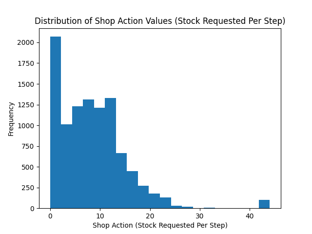
Here we see that the shop most commonly requests just over 25 units of stock each step.

This is a logical value as the 5 customers each requesting 5 units of product each step gives an average order rate of 25.

# Plot distribution of shop action (stock request) per step for all rollouts
plt.hist(shop_actions, bins=20)
plt.title("Distribution of Shop Action Values (Stock Requested Per Step)")
plt.xlabel("Shop Action (Stock Requested Per Step)")
plt.ylabel("Frequency")
plt.savefig("supply_chain_shop_action_values.png")
plt.close()

Here we see that the stock held by shop is most commonly just over 25 units.

Depending on the variation in size of recent orders it may be less or more.

plt.hist(shop_stock, bins=20)
plt.title("Distribution of Shop Held Stock")
plt.xlabel("Shop Held Stock (Per Step)")
plt.ylabel("Frequency")
plt.savefig("supply_chain_shop_held_stock.png")
plt.close()

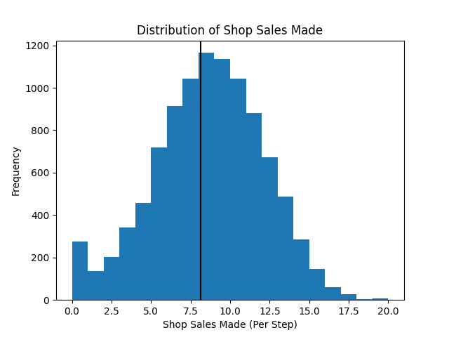
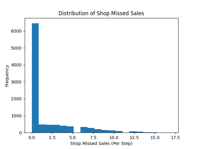
In the next plot we see that the average shop sales per step is just under the average of 25 orders placed per step.

In the second plot we see that as a result of this there is a small amount of steps in which the shop fails to fulfil all orders.

plt.hist(shop_sales, bins=20)
plt.axvline(np.mean(shop_sales), c="k")
plt.title("Distribution of Shop Sales Made")
plt.xlabel("Shop Sales Made (Per Step)")
plt.ylabel("Frequency")
plt.savefig("supply_chain_shop_sales_made.png")
plt.close()

plt.hist(shop_missed_sales, bins=20)
plt.title("Distribution of Shop Missed Sales")
plt.xlabel("Shop Missed Sales (Per Step)")
plt.ylabel("Frequency")
plt.savefig("supply_chain_shop_missed_sales.png")
plt.close()